Tutorial
We begin by loading numpy, matplotlib.pyplot and BayesPowerlaw:
import numpy as np
import matplotlib.pyplot as plt
import BayesPowerlaw as bp
Next we simulate a single power law distribution using the power_law function:
#define variables for simulation
exponents=[2.0]
weights=[1.0]
sample_size=1000
xmax=10000
#simulate data following power law distribution
data = bp.power_law(exponents,weights,xmax,sample_size)
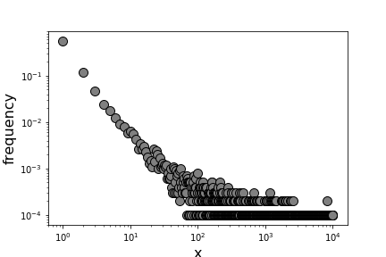
We can simply plot the data by running the bayes function while specifying that we don’t want to perform the fitting:
#create a bayes-data object without fitting
bayes_object = bp.bayes(data, fit=False)
#plot the distribution without the fit

plt.figure(figsize=(6,4))
bayes_object.plot_fit(1.01,scatter_size=100,data_color='gray',edge_color='black',fit=False)
plt.xlabel('x', fontsize=16)
plt.ylabel('frequency',fontsize=16)

Let’s perform the fitting of the simulated power law and get an exponent. This can take up to 30s, depending on your hardware specs:
#perform the fitting
fit=bp.bayes(data)
#get the posterior of exponent attribute. Since we only have a singular power law, we need only the first (index = 0) row of the 2D array.
posterior=fit.gamma_posterior[0]
#mean of the posterior is our estimated exponent
est_exponent=np.mean(posterior)
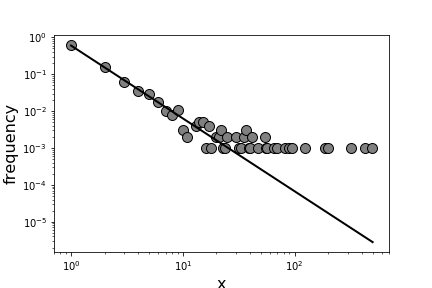
Now let’s plot the distribution with the fit:
plt.figure(figsize=(6,4))
fit.plot_fit(est_exponent,fit_color='black',scatter_size=100,data_color='gray',edge_color='black',line_width=2)
plt.xlabel('x', fontsize=16)
plt.ylabel('frequency',fontsize=16)
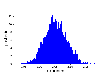
We can also plot the posterior distribution:
plt.figure()
fit.plot_posterior(posterior,color='blue')
plt.xlabel('exponent', fontsize=16)
plt.ylabel('posterior',fontsize=16)
To simulate a mixed power law distribution, input multiple exponents and their corresponding weights:
#define variables for simulation
exponents=[1.1,2.5]
weights=[0.3,0.7]
sample_size=10000
xmax=10000
#simulate data following power law distribution
data = bp.power_law(exponents,weights,xmax,sample_size)
Let’s plot the simulated mixed power law using bayes function:
#create a bayes-data object without fitting
bayes_object = bp.bayes(data, fit=False)
#plot the distribution without the fit
plt.figure(figsize=(6,4))
bayes_object.plot_fit(1.01,scatter_size=100,data_color='gray',edge_color='black',fit=False)
plt.xlabel('x', fontsize=16)
plt.ylabel('frequency',fontsize=16)
To fit a mixture of power law, specify how many power laws are in the mixture. This may take some time:
#perform the fitting
fit=bp.bayes(data,mixed=2)
#get the posterior of exponent attribute. Since we have a mixture of 2 power laws, we need 2 rows (index=0 and 1) of the 2D array.
posterior1=fit.gamma_posterior[0]
posterior2=fit.gamma_posterior[1]
#also, get the weight posteriors corresponding to exponents.
weight1=fit.weight_posterior[0]
weight2=fit.weight_posterior[1]
#mean of the posterior is our estimated exponent and weight.
est_exponent1=np.mean(posterior1)
est_exponent2=np.mean(posterior2)
est_weight1=np.mean(weight1)
est_weight2=np.mean(weight2)
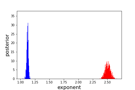
Let’s plot the posterior distributions of the exponent and weight
plt.figure()
fit.plot_posterior(posterior1,color='blue')
fit.plot_posterior(posterior2,color='red')
plt.xlabel('exponent', fontsize=16)
plt.ylabel('posterior',fontsize=16)

plt.figure()
fit.plot_posterior(weight1,color='blue')
fit.plot_posterior(weight2,color='red')
plt.xlabel('weight', fontsize=16)
plt.ylabel('posterior',fontsize=16)
plt.xlim([0,1])
Note, correct answers for exponent are 1.1 and 2.5. Correct answers for weights are 0.3 and 0.7 respectively.